Network Analysis

Goals and Objectives:

 

 

The goal of this lab was to learn and perform network analysis to figure out the economic impact of trucking sand to and from sand mines to rail road terminals. Per usual for the class, Trempealeau County has a focus. A script was created first to select the mines that met the requirements. Then network analysis was performed to figure the best route for each mine to its closest terminal. From there I figured with the truck routes and estimated cost per mile I determined a hypothetical economic impact on the roads in each county for mining in Wisconsin. Much of this was done using model builder.

Methods:

The first part of this lab was to create a script in order to select the suitable mines, you can find more details below in Post 2, or click here.

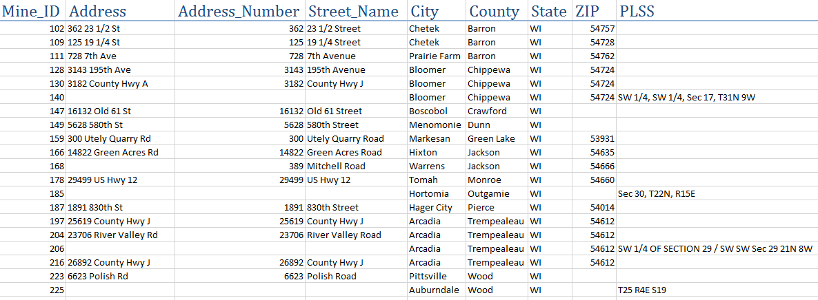
First I connected to ESRI's originalrawdata2013\streetmap_na\data and added the "streets" data to ArcMap. I also added the rail terminal data and mines terminal data provided by my professor. I had to select only the terminals that strictly had RAIL in the MODE_TYPE field, ensuring that none used any other form of transportation. Then using the network analysis toolbar and extension I set up a closest facility layer and set the mines as the "incidents" and the rail terminals as "facilities," then solved for closest facility.

After deleting the address field in my mines feature class (it causes a problem in model builder) I opened up model builder to create a data flow model, seen in Figure A. First I added streets to the Make Closest Facility layer tool and set it to "Travel To Facility," then using the Add Locations tool I added mines and final rail terminals. After adding the Solve tool, I ran the model. Using the Select Data tool and Copy Features tool I now have my best route in my geodatabase.

Everything from here on is done to determine the total distance traveled on the roads in each county and the cost of road maintenance annually for each county. First I projected my routes and my Wisconsin counties into the NAD 1983 HARN Transverse Mercator (meters) coordinate system, then I intersected the the routes and Wisconsin counties. Next I need used the Add Field tool to create a new field which I called Distance. Then using the Calculate Field tool I changed the distance of the routes from meters to miles using the equation [SHAPE_LENGTH] * .000621371, (1 meter = .000621371 miles). Using the Add Field tool again I created a field and named it Annual_Cost. Again using the Calculate Field tool and using the equation [Distance] *50 *2 *.022 I found the cost per year of each segment of road that was being driven on. Making assumptions our professor instructed us to use 50 as the amount of times annually that each mine trucks sand, multiplied by 2 because the trucks have to come back to the mine, and that it costs 2.2 cents each mile. The last step was to use the Summarize Statistics tool to create a table that had contained each county, and its annual miles driven by the trucks on the routes, and the annual cost.

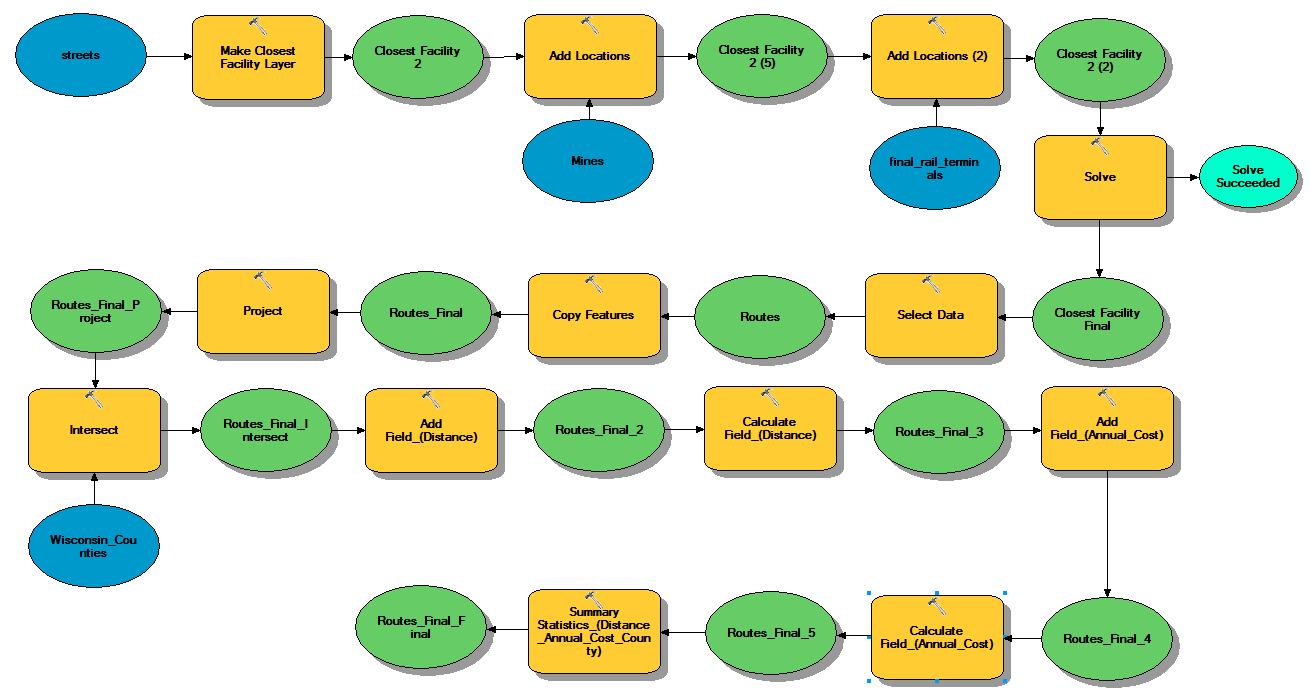Figure A shows my workflow for the exercise created in model builder.

Results:

A total of 19 counties in the state of Wisconsin have sand mines that fit the criteria. The roads in these counties are affected by the trucking of sand, some worse than others, in terms of hypothetical annual cost. Using network analysis I was able to see how often the roads were traveled and although the numbers and dollars are speculations, that does not mean that this is meaningless because it still shows which states and roads are seeing more travel than others.

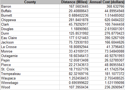Figure B shows the total distance the trucks traveled and the annual cost for each of the 19 counties.

 

Figure C shows the truck mileage per county. Due to county lines Waupaca, Winnebago, and Burnett have very little miles. Much in contrast to Chippewa and Eau Claire counties.

Figure D shows the annual costs each county would spend to repair the roads. Chippewa county would spend nearly double the next closest, Eau Claire County.

Figure D shows the locations of mines, rail terminals, and the truck routes. The counties scale from light to dark brown, lower annual cost to higher annual cost respectively.

Discussion:

The costs on average were less than I had expected, but simultaneously I did not expect to have some values be so low, Burnett, Douglass, Waupaca, and Winnebago counties. These costs while they may be reflective, could be wildly inaccurate because we assumed 50 trips per year, some mines may do more and some may do less. We also assumed the cost to be 2.2 cents per mile, this may increase or decrease as the economic state of Wisconsin shifts. We also did not bring in to consideration the type of roads, because some types roads wither more easily than others due to their make up. 

Another fallacy with our accuracy is that our network analysis techniques only calculate the most time efficient route from the mine to the rail, that time efficient route may not be the best route. And the data is from at least two years ago, I doubt many roads have changed, but in the last two years new roads could have been constructed that would make better pathways.

Conclusion:

I learned a lot from this exercise, most notably I learned how to do network analysis, which is a very key and integral part of GIS. I was also exposed to model builder again, I had previous but limited exposure to in in GIS 1, which was also a year ago.

Sources:

Hart, M. V., Adam, T., Schwartz, A. (2013). Transportation Impacts of Frac Sand Mining in the MAFC Region: Chippewa County Case Study. National Center for Freight & Infrastructure Research & Educatoin, White Paper Series: 2013, Retrieved  November 19, 2015 from http://midamericafreight.org/wpcontent/uploads/FracSandWhitePaperDRAFT.pdf

Dr. Christina Hupy

ESRI street map USA

Wisconsin Department of Natural Resources

Data Normalization, Geocoding, and Error Assessment

Goals and Objectives:

The goal of this lab was to geocode the locations of our sand mines in Wisconsin. Each Student had to geocode 21 different mines, because of overlap each mine was geocoded by at least 3 different people. The next goal was to compare positional accuracy of our mines to our classmates mines and the actual location of the mines provided by our professor.

Methods:

We were provided with a table (from the WI DNR) containing a lot of information about all of the frac sand mines in Wisconsin, including but not limited to owners, addresses, counties, zip code, etc. as seen below in Figure A. I had to find the mines I was responsible for and create a normalized table from the information given. The normalized table, created in Excel can be seen below, Figure B. The normalized table was important because it separated the addresses, zip codes, City, State and in some cases PLSS information. From there I added the table into ArcMap; using the Geocoding Addresses dialog box I created a shape file out of it. In order to do so I used my UWEC information to log into an Enterprise Account and geocode the addresses using the World Geocode Service. 16 of the addresses from the table had matches in the geocoding process, the other 5 were unable to be processed from the given information, this required further inspection and finding the addresses myself.

The of the 5 addresses that were incorrect, were incorrect because the addresses was unidentifiable or because the information given was in PLSS (Public Land Survey System) format. Using a basemap in ArcMap, the address inspector function, and Google Maps I was able to find the location of these mines and select their point for my shape file. When I was selecting the locations, I made sure to select what I believed to be the correct address based on the information I was given, and I also made my point as close to the road system to ensure best accuracy.

Figure A: Table provided by the WI DNR containing a plethora of not normalized information about each mine.

Figure B: My normalized Excel table of the mines I was responsible for.

Once all geocoding was complete I added my shape file and the shape files of my 3 classmates who geocoded mines with the same Mine Unique ID as mine. Between those three all of mine were accounted for and I was able to compare the positional accuracy for all of my mines. To do this I had to first project all of our shape files into a different coordinate system because I needed my distances in meters, not in decimal degrees. Using the project tool, I changed them all to WGS_1984_World_Mercator projected coordinate system. Then I used the Near Tool to calculate the distances between my mines and my 3 classmates mines; these can be seen below in Figures D, E, and F. After that was completed I did the exact same thing with the actual mine locations provided by my professor in a shape file, these results can be seen in below in Figure G.

Results:

Figure C: Shows the location of my geogoded mines (red) compared to the actual mine location (blue).

Figure D: Shows the distances between some of my mines and one of my classmates mines. Larger numbers (meters) indicate higher discrepancies between my geocoding and theirs. The average distance between our points is 7,342 meters.

Figure E: Shows the distances between some of my mines and one of my classmates mines. Larger numbers (meters) indicate higher discrepancies between my geocoding and theirs. The average distance between our points is 434 meters.

Figure F: Shows the distances between some of my mines and one of my classmates mines. Larger numbers (meters) indicate higher discrepancies between my geocoding and theirs. The average distance between our points is 4,216 meters.

Figure G: Shows the distances between my mines and the actual mine locations. Larger numbers (meters) indicate higher discrepancies between in my geocoding. The average distance between my points and the actual points is 5,166 meters.

Discussion:

The accuracy between my results and the results of my three peers was on average, 3,997 meters apart. The average distance between my mines and the actual mine locations, as seen above in Figure G, was 5,166 meters. Errors in accuracy could have been caused by many different factors and mistakes made by myself and my classmates. A possible error may have occurred in the field, the survey crew who recorded the location of the mine may have placed the point in the center of the mine and my point was placed at the road, or nearest to the exit. Another mistake could have been made when geocoding. The geocoding tool uses and actual address, and that address point on the map may not accurately reflect the location of the mine. Lastly, when geocoding for mines when I did not have a specific address I used the the basemap, Google Maps, and the PLSS information. When using these aerial views I may have selected a mine that was incorrect or possibly not even selected a mine at all because the aerial maps could have been outdated.

Conclusion:

This lab was very good at portraying how difficult and easy geocoding can be simultaneously. ArcMap has great tools to help geocoding go smoothly, but unless all the requirements are met correctly, it can be a real pain. It was also a learning experience having to deal with other people's data, because there can be many difficulties that come with it. Normalization is now a concept I understand much better, and have a firmer grasp on. All in all it was a good learning experience normalizing data, geocoding, and finding accuracy with my datasets and my peers.