Monday, December 14, 2015

Sand Mine Suitability Using Raster Analysis


Goals and Objectives:

The goal of this lab was to use various raster geoprocessing tools to build models for both sand mining suitability and environmental and cultural risk in Trempealeau County, WI. Using different tools such as, Reclassify, Euclidian Distance, project, polygon to raster, slope, block statistics, and raster calculator, and using different raster layers such as, DEM (digital elevation model), land use and land cover datasets, and geology I was able to look at the suitability of the land as well as the impact a mine would have. I created two different data flow models, one for land suitability, and the other for risk assessment, using raster calculator I was able to put these two together to create a location index. The index being a collaboration between my two final criteria shows where sand mines should be created to minimize impact and maximize suitability.

Methods:

SUSTAINABILITY MODEL

I was given 5 variables that are considered important when finding suitability:
  1. Geology
  2. Land Use Type
  3. Proximity to Railroad Terminals
  4. Slope of the ground
  5. Water Table Depth
The data I had available through previous labs and downloading (water table depths) was not all in raster format. After transforming my data into raster, I needed to rank my data based on how important it would be to sustainability and risk. The ranking was of 1-3, 1 having low suitability/high risk and 3 having high suitability/high risk (a rank of 2 was somewhere in between). In two instances (geology and land use) the rank of 0 was given, this is because the geology was not silica sand bearing geology and the land use was water (Figure A below).


Figure A shows the rankings and values in each category that correspond with the ranking system.


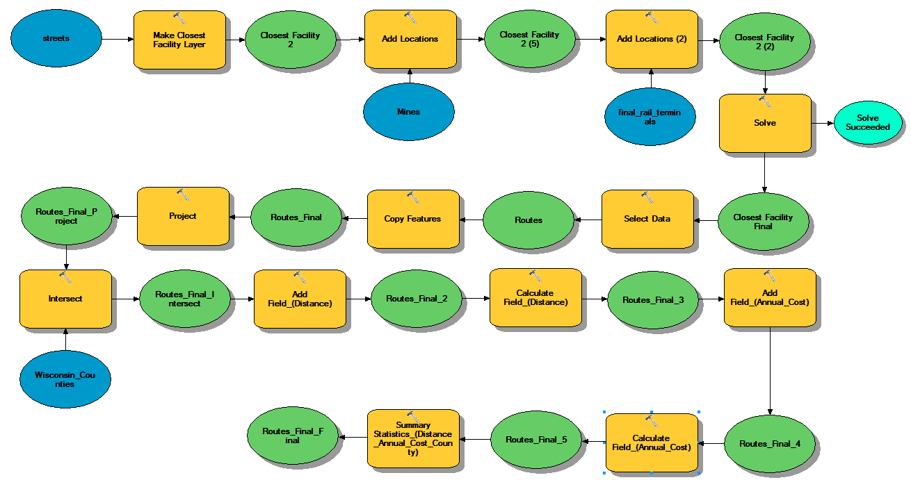
You can see below in Figure B, that each variable was modified using a series of tools to analyze the data and create rasters. The rasters were then all combined using raster calculator to create the final Suitability map.


Figure B is my data flow model to determine the suitability of an area for Frac Sand Mining.


Geology: The Jordan and Wonewaoc formations were selected for sand mining, these were given a ranking of 3, while all other geologic formations received a 0. Figure C is the result. Land Use: Based on what was most practical, it would not be practical or possible to put a sand mine on a lake or on water or in a developed area, these were removed by classifying them as NoData. Figure D is the result. Railroads: The railroads were ranked on how far away the mine was from the rail terminal. The further the distance the lower the ranking for suitability, because trucking sand long distances costs money and can damage the roads. See Figure E. Slope: Slope ranking was based on how steep the slow is for an area. Steeper slopes are given a lower ranking because it would be more difficult and time consuming to build a sand mine on a steep slope. See Figure F. Water Table: Ranking based on how deep the water is in the ground. If the water table was closer to the surface, it was given a higher ranking because of accessibility. See Figure G.


Figure C.


Figure D.


Figure E.


Figure F.


Figure G.
IMPACT MODEL


I was given 4 variables to use to determine how a mine would impact an area. The 5th variable I got go choose.
  1. Streams
  2. Prime Farmland
  3. Residential proximity
  4. Schools
  5. Bike Trails
Seen below in Figure H each variable was modified using a series of tools to analyze the data and create rasters. The rasters were then all combined using raster calculator to create the final Impact map.


Figure H is my data flow model to determine the impact on the area of a Frac Sand Mine.

Streams: streams located near sand mines could potentially be negatively impacted by runoff and cause a loss of wildlife. A higher ranking is awarded the further away from the stream an area is. Only certain streams were selected, those with an order greater than 2, this means they flow more and year round. Seen below in Figure IPrime Farmland: it is better to find mining sites that are not on prime farmland; therefore, areas of poor farmland were given a higher ranking than areas with prime farmland, seen in Figure J. Residential areas: land further away from residential areas was given a higher ranking than land closer to residential areas. This is because mines produce dust and noise, both of which are not favoured near peoples' homes, Figure K. Schools: having a mine near a school could result in both class disruption from noise and children's health due to dust particles. Land further from a school received a higher ranking than land closer to a school, seen below in Figure L. Bike trails: land further from bike trails received a higher ranking than land closer to bike trails. This is because biking takes a lot of energy and breath, if someone is biking it could be dangerous to their health to have a sand mine too close to the trail. Also people go on bike trails for the beautiful scenery, a sand mine might destroy that. Results shown in Figure M below.


Figure I.
Figure J.
Figure K.
Figure L.
Figure M.
Results:
The results of the mining suitability data flow model can be seen below in Figure N. Areas with a higher number are areas that are more suitable for sand mining. The results for the Impact data flow model can be seen in Figure O. A higher number on this map corresponds with a lower impact. On BOTH maps a higher number shows a better area to put a mine.


Figure N. The southern part of the county is more suitable for sand mining
Figure O. High impact/risk areas are spread evenly throughout the state.


Below Figure P is the combined output of both maps. It uses criteria from both maps to create a map that shows the prime areas to put sand mines, and the worst areas to sand mines.

Figure P.
Discussion:

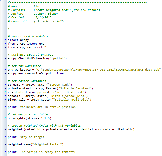
From Figure P it is easy to tell which areas are more suitable and would have the least amount of risk/impact associated with putting a sand mine in an area. The final map could use some improvements before it would be used in a real situation. If the map was going to be used by professionals it would need more detail of the qualities of land in the farmland and land use departments, because that data is from 2011 which is nearly 5 years ago now. An update in data would potentially change the outcome of the ranking system to better show real life conditions. In my model all of the variables carry the same weight, this would not be the case in the real world, certain things may be more important, like streams for example, this would change the outcome of the map. This is shown by the Python Script I had to do for the other part of the lab.

Conclusions:

I learned a lot about the spatial analysis tools and rasters while doing this lab, in particular the reclassify and Euclidian distance tools. This lab and the previous lab really focused on the evaluation of sand mining and have been very useful for me in learning and mastering GIS. These skills, maps, and practices can be very helpful for the mining industry and local governments as they construct mines and regulate policies.

Sources:

Wisconsin Geological and Natural History Survey (GNHS). Water table contours. GIS data. (n.d). Retrieved December 6, 2015, from http://wgnhs.uwex.edu/map-data/gis-data/

 Wisconsin Geological and Natural History Survey (WGNHS). B.A. Brown, 1988. Bedrock Geology of Wisconsin, West-Central Sheet, WGNHS Map 104. Digitizing by Beatriz Vidru Linhares, University of Wisconsin Eau Claire (UWEC). Retrieved from UWEC GIS resources.

Bureau of Transportation Statistics. (n.d.). Rail terminals feature class. Retrieved December 6, 2015, from http://www.rita.dot.gov/bts/sites/rita.dot.gov.bts/files/subject_areas/geographic_information_services/index.html


 Land Records. (n.d.). Trempealeau County Land Records. Geodatabase. Retrieved December 6, 2015, from http://www.tremplocounty.com/landrecords/


United States Geological Survey, National Map Viewer. National Land Cover Database (NLCD) raster and DEM. (n.d). Retrieved December 6, 2015, from http://nationalmap.gov/viewer.html

Wednesday, November 25, 2015

Network Analysis

Goals and Objectives:
 
 
The goal of this lab was to learn and perform network analysis to figure out the economic impact of trucking sand to and from sand mines to rail road terminals. Per usual for the class, Trempealeau County has a focus. A script was created first to select the mines that met the requirements. Then network analysis was performed to figure the best route for each mine to its closest terminal. From there I figured with the truck routes and estimated cost per mile I determined a hypothetical economic impact on the roads in each county for mining in Wisconsin. Much of this was done using model builder.

Methods:


The first part of this lab was to create a script in order to select the suitable mines, you can find more details below in Post 2, or click here.


First I connected to ESRI's originalrawdata2013\streetmap_na\data and added the "streets" data to ArcMap. I also added the rail terminal data and mines terminal data provided by my professor. I had to select only the terminals that strictly had RAIL in the MODE_TYPE field, ensuring that none used any other form of transportation. Then using the network analysis toolbar and extension I set up a closest facility layer and set the mines as the "incidents" and the rail terminals as "facilities," then solved for closest facility.


After deleting the address field in my mines feature class (it causes a problem in model builder) I opened up model builder to create a data flow model, seen in Figure A. First I added streets to the Make Closest Facility layer tool and set it to "Travel To Facility," then using the Add Locations tool I added mines and final rail terminals. After adding the Solve tool, I ran the model. Using the Select Data tool and Copy Features tool I now have my best route in my geodatabase.


Everything from here on is done to determine the total distance traveled on the roads in each county and the cost of road maintenance annually for each county. First I projected my routes and my Wisconsin counties into the NAD 1983 HARN Transverse Mercator (meters) coordinate system, then I intersected the the routes and Wisconsin counties. Next I need used the Add Field tool to create a new field which I called Distance. Then using the Calculate Field tool I changed the distance of the routes from meters to miles using the equation [SHAPE_LENGTH] * .000621371, (1 meter = .000621371 miles). Using the Add Field tool again I created a field and named it Annual_Cost. Again using the Calculate Field tool and using the equation [Distance] *50 *2 *.022 I found the cost per year of each segment of road that was being driven on. Making assumptions our professor instructed us to use 50 as the amount of times annually that each mine trucks sand, multiplied by 2 because the trucks have to come back to the mine, and that it costs 2.2 cents each mile. The last step was to use the Summarize Statistics tool to create a table that had contained each county, and its annual miles driven by the trucks on the routes, and the annual cost.


Figure A shows my workflow for the exercise created in model builder.

Results:

A total of 19 counties in the state of Wisconsin have sand mines that fit the criteria. The roads in these counties are affected by the trucking of sand, some worse than others, in terms of hypothetical annual cost. Using network analysis I was able to see how often the roads were traveled and although the numbers and dollars are speculations, that does not mean that this is meaningless because it still shows which states and roads are seeing more travel than others.


Figure B shows the total distance the trucks traveled and the annual cost for each of the 19 counties.
 
Figure C shows the truck mileage per county. Due to county lines Waupaca, Winnebago, and Burnett have very little miles. Much in contrast to Chippewa and Eau Claire counties.


Figure D shows the annual costs each county would spend to repair the roads. Chippewa county would spend nearly double the next closest, Eau Claire County.
Figure D shows the locations of mines, rail terminals, and the truck routes. The counties scale from light to dark brown, lower annual cost to higher annual cost respectively.


Discussion:

The costs on average were less than I had expected, but simultaneously I did not expect to have some values be so low, Burnett, Douglass, Waupaca, and Winnebago counties. These costs while they may be reflective, could be wildly inaccurate because we assumed 50 trips per year, some mines may do more and some may do less. We also assumed the cost to be 2.2 cents per mile, this may increase or decrease as the economic state of Wisconsin shifts. We also did not bring in to consideration the type of roads, because some types roads wither more easily than others due to their make up. 

Another fallacy with our accuracy is that our network analysis techniques only calculate the most time efficient route from the mine to the rail, that time efficient route may not be the best route. And the data is from at least two years ago, I doubt many roads have changed, but in the last two years new roads could have been constructed that would make better pathways.

Conclusion:

I learned a lot from this exercise, most notably I learned how to do network analysis, which is a very key and integral part of GIS. I was also exposed to model builder again, I had previous but limited exposure to in in GIS 1, which was also a year ago.

Sources:

Hart, M. V., Adam, T., Schwartz, A. (2013). Transportation Impacts of Frac Sand Mining in the MAFC Region: Chippewa County Case Study. National Center for Freight & Infrastructure Research & Educatoin, White Paper Series: 2013, Retrieved  November 19, 2015 from http://midamericafreight.org/wpcontent/uploads/FracSandWhitePaperDRAFT.pdf

Dr. Christina Hupy

ESRI street map USA

Wisconsin Department of Natural Resources

Monday, November 16, 2015

Data Normalization, Geocoding, and Error Assessment

Goals and Objectives:

The goal of this lab was to geocode the locations of our sand mines in Wisconsin. Each Student had to geocode 21 different mines, because of overlap each mine was geocoded by at least 3 different people. The next goal was to compare positional accuracy of our mines to our classmates mines and the actual location of the mines provided by our professor.

Methods:

We were provided with a table (from the WI DNR) containing a lot of information about all of the frac sand mines in Wisconsin, including but not limited to owners, addresses, counties, zip code, etc. as seen below in Figure A. I had to find the mines I was responsible for and create a normalized table from the information given. The normalized table, created in Excel can be seen below, Figure B. The normalized table was important because it separated the addresses, zip codes, City, State and in some cases PLSS information. From there I added the table into ArcMap; using the Geocoding Addresses dialog box I created a shape file out of it. In order to do so I used my UWEC information to log into an Enterprise Account and geocode the addresses using the World Geocode Service. 16 of the addresses from the table had matches in the geocoding process, the other 5 were unable to be processed from the given information, this required further inspection and finding the addresses myself.

The of the 5 addresses that were incorrect, were incorrect because the addresses was unidentifiable or because the information given was in PLSS (Public Land Survey System) format. Using a basemap in ArcMap, the address inspector function, and Google Maps I was able to find the location of these mines and select their point for my shape file. When I was selecting the locations, I made sure to select what I believed to be the correct address based on the information I was given, and I also made my point as close to the road system to ensure best accuracy.

Figure A: Table provided by the WI DNR containing a plethora of not normalized information about each mine.


Figure B: My normalized Excel table of the mines I was responsible for.

Once all geocoding was complete I added my shape file and the shape files of my 3 classmates who geocoded mines with the same Mine Unique ID as mine. Between those three all of mine were accounted for and I was able to compare the positional accuracy for all of my mines. To do this I had to first project all of our shape files into a different coordinate system because I needed my distances in meters, not in decimal degrees. Using the project tool, I changed them all to WGS_1984_World_Mercator projected coordinate system. Then I used the Near Tool to calculate the distances between my mines and my 3 classmates mines; these can be seen below in Figures D, E, and F. After that was completed I did the exact same thing with the actual mine locations provided by my professor in a shape file, these results can be seen in below in Figure G.

Results:
Figure C: Shows the location of my geogoded mines (red) compared to the actual mine location (blue).

Figure D: Shows the distances between some of my mines and one of my classmates mines. Larger numbers (meters) indicate higher discrepancies between my geocoding and theirs. The average distance between our points is 7,342 meters.
Figure EShows the distances between some of my mines and one of my classmates mines. Larger numbers (meters) indicate higher discrepancies between my geocoding and theirs. The average distance between our points is 434 meters.

Figure FShows the distances between some of my mines and one of my classmates mines. Larger numbers (meters) indicate higher discrepancies between my geocoding and theirs. The average distance between our points is 4,216 meters.

Figure GShows the distances between my mines and the actual mine locations. Larger numbers (meters) indicate higher discrepancies between in my geocoding. The average distance between my points and the actual points is 5,166 meters.

Discussion:

The accuracy between my results and the results of my three peers was on average, 3,997 meters apart. The average distance between my mines and the actual mine locations, as seen above in Figure G, was 5,166 meters. Errors in accuracy could have been caused by many different factors and mistakes made by myself and my classmates. A possible error may have occurred in the field, the survey crew who recorded the location of the mine may have placed the point in the center of the mine and my point was placed at the road, or nearest to the exit. Another mistake could have been made when geocoding. The geocoding tool uses and actual address, and that address point on the map may not accurately reflect the location of the mine. Lastly, when geocoding for mines when I did not have a specific address I used the the basemap, Google Maps, and the PLSS information. When using these aerial views I may have selected a mine that was incorrect or possibly not even selected a mine at all because the aerial maps could have been outdated.

Conclusion:

This lab was very good at portraying how difficult and easy geocoding can be simultaneously. ArcMap has great tools to help geocoding go smoothly, but unless all the requirements are met correctly, it can be a real pain. It was also a learning experience having to deal with other people's data, because there can be many difficulties that come with it. Normalization is now a concept I understand much better, and have a firmer grasp on. All in all it was a good learning experience normalizing data, geocoding, and finding accuracy with my datasets and my peers.

Friday, October 23, 2015

Gathering Data and Assessing Accuracy

Goals and Objectives:

The goal of this lab was to familiarize myself with the process of gathering and downloading data from different organizations on the internet. After the data was gathered I had to import it into ArcGIS and project it from all of its different sources into a single common coordinate system. I also had to design a getodatabase to store all the data; this had to be done by writing python scripts in PyScripter. You can view my scripts here. The challenge of this lab was writing script that would actually work, as well as keeping all the downloaded data organized and easily accessible. Like all the posts/labs in this blog they share the common goal to build a risk and sustainability model for sand mining in western Wisconsin. All of the data downloaded for this lab was focused on Tremealeau County for purposes of proximity and to minimized the sheer amount of data stored.

Methods:

The first step in this lab was to obtain our data from the internet (Figure A) . Below is a list of the specified data sources required for this lab.


Figure A: a basic work flow created by Professor Hupy provided for us in our instructions.

All the datasets were downloaded to a temporary file, they were then unzipped, extracted, to a working folder. I downloaded them to a temporary file first in order to save storage space, the temporary files are deleted from the system at the end of every month. Then we sorted our files, choosing the files we needed: railroad feature class, soils information, DEM elevation rasters, and national land use and land cover data. These were all sent to a master folder along with the TMP geodatabase. As mentioned before this data was used in the next step, the coding process in python.

The data (the four listed above) was then projeted into the same coordinate system as the TMP geodatabase, NAD83_HARN_WISCRS Trempealeau County Feet. It was then clipped to the Trempealeau County boundary. Finally it was loaded to the geodatabase and we were able to use it effectively, and create some maps. After all was said and done all unnecessary and redundant data was deleted.

Data Accuracy:

Using the metadata from each dataset I was able to investigate the accuracy of said data. This is very important because our data came from many different sources and therefore it would have varying degrees of accuracy. Delving into the depths of the metadata has helped me better understand where the data is from, how frequently it is kept up to date, who has accessed it, its resolution, etc. In figure B below you can see the accuracy for each dataset.

Figure B: Data Quality Table
NA represents data that was unavailable or that I could not locate.

Conclusion:

I learned how to download and organize a ridiculous amount of data from different sources, probably minuscule compared to professional level GIS users, but I digress. I feel like this is a great skill to have learned and to now hone. I also learned a lot about metadata and the data itself, it was endearing, but worth it, I feel smarter now. Using python to do things in Arc is a great skill to have begun learning because it will prove to be very helpful.


Post 2: Python Script

Python is a coding software that is integrated with Arc, it helps users perform tasks in Arc with less error, more efficiency, and to make life a little bit easier. As we use PyScriptor more I will update this post with more screenshots of script used for GIS2.

Script 1:
In part two of lab 5 we wrote our first python script (after a week or so of practicing in class). The purpose was to project 3 rasters, a DEM, a land cover, and a cropland, then clipped using extract by mask, and finally loaded into a geodatabase. Below is a screenshot of my script.


Script 2:
This script was made to select mines from the all_mines feature class, provided by our professor, that contained only mines in Wisconsin. I also only selected mines that are active and greater that 1.5 km from a rail road system. With these in place we can better understand which mines have to transport their sand to and from mines via trucks.


Script 3:
The last script of the semester takes the rasters I made in EX8 for the risk/impact assessment and creates a weighted index from them. The output of the python script is the same as the output of the calculate raster tool for the risk/impact part of EX8, except that in my scenario, the streams is weighted more than the others.


Thursday, October 22, 2015

Frac Sand Mining in Western Wisconsin: An Overview

In the past few years you could hardly go anywhere in U.S., especially Wisconsin, without hearing about fracing. The word sounds almost inappropriate, but I assure you, it isn't. More specifically it is called Hydraulic Fracturing, Hydrofracking for short, and it is a method used to extract resources, most notably natural gas. A well is drilled and explosives are detonated in the earth to create cavities. A mixture of water, sand, and chemicals are pumped down in the well under high pressures to keep the cracks maintained while the natural gas, or other resource is being removed (Figure A).
Figure A: Hydraulic Fracturing Illustrated
http://www.candcworldwide.com/ckfinder/userfiles/images/Fracking-diagram.jpg
This technique is nothing new, it has been in use for roughly sixty years; however, it has found its way into a new territories because of technological advancements. People want to drill for resources where they previously could not, an increase in hydrofracking means they're going to need more hyrdrofracking components, which is where Wisconsin comes in! Of course the best frac sand comes from the best of all 50 states, it's only natural. In 2014 Wisconsin was the leading producer of Frac Sand. This frac sand (quartz sand or silica sand, it's all the same) is so great for hydraulic fracturing because it is almost entirely quartz, very round, and uniformly sized (Figure B). This sand can be found in Cambrian Sandstone formations which are readily available in areas of western Wisconsin (Figure C). Mining of quartz sand in Wisconsin is found primary in the western portion including Monroe, Jackson, Burnett, Chippewa, and Trempealeau counties (Figure D). 
Figure B: Frac Sand on a penny
http://apps.startribune.com/blogs/user_images/sand2.JPG


Figure C: Red areas show the Cambrian Sandstone in Wisconsin
Full image: http://u6efc47qb7f1g5v06kf9kfdcn.wpengine.netdna-cdn.com/wp-content/uploads/2012/01/Where-the-best-sand-is-Brown-presentation.jpg


Figure D: Sand mines in Wisconsin
http://glaciersands.com/wp-content/uploads/2012/05/sandwi-large.png

There are seven steps in processing frac sand:

  1. Overburden removal: Removal of everything unwanted above the sand at the site.
  2. Excavation: Systematically dig a pit.
  3. Blasting: Breaking apart the heavily cemented sandstone with dynamite.
  4. Crushing: Larger pieces of sandstone moved and broken down into grains.
  5. Processing: washing, drying, sorting, and storing of the grains to ensure sand is uniform and clean of contaminants.
  6. Transporting: Sand is sent to hydraulic fracturing sites, by truck or by train.
  7. Reclamation: Reclaiming the land after the sand has been removed. Including but not limited to: replacing soil, planting trees, making the land usable for farm or commercial use.

Sand mining uses many resources throughout the entire process including the burning of fossil fuels to power machinery and using groundwater to wash the grains and spray down the dirt and sand piles in order to reduce particulates in the air. Trucks moving sand will damage the roads and cause lots of noise, not nearly as much as the massive machinery and explosives though. The removal of millions of tons of earth will leave the landscape looking lack luster even after reclamation, and possibly leave lasting negative effects on the environment. On the bright side sand mines provide jobs, stimulate the local economy, and potentially lower the cost of natural gas. Throughout the rest of the semester we will use GIS to analyze sand mines and gain better understanding of how they operate. We also aim to add a level of sustainability to the known sand mines.

Sources:

Frac Sand Mining Fact Sheet
http://wcwrpc.org/frac-sand-factsheet.pdf

Wisconsin Department of Natural Resources. (January 2012). Silica Sand Mining in Wisconsin
http://dnr.wi.gov/topic/Mines/documents/SilicaSandMiningFinal.pdf

Thomas Content. Journel Sentinel. (May 2015). Wisconsin's frac sand industry booms